2.5 State set

According to the definition of cellular automata, each cell is a finite automaton, and therefore the set of states has finite size. In addition, the set is usually fairly small. There are several reasons for this. People have investigated all possible CAs with a given number of states and a given neighborhood size [7]. This is only possible when the set of states is very small, since the number of possible CAs with $s$ states and $n$ cells in the neighborhood (including the cell to be updated), is $s^{s^n}$. This number rapidly becomes too big to explore all possibilities as $n$ and $s$ grow:

$$\begin{array}{cccc} s & n & s^n & s^{s^n} \\ 2 & 3 & 8 & 256\\... ... 32 & 4294967296\\ 5 & 3 & 125 & 2.3 \cdot 10^{87}\\ \end{array}$$

The second reason to prefer small state sets, and which is more important for simulation, is that only when there are few states is it possible to specify the CA rules explicitly and store them in a table (the table size is $s^n$)

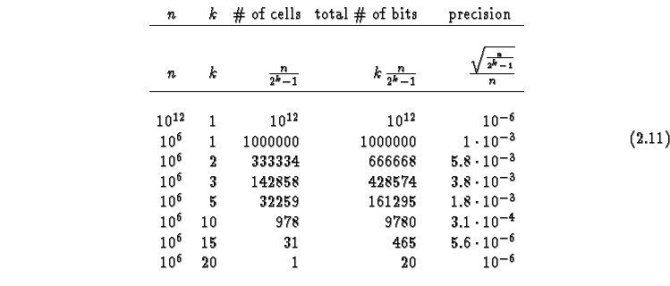
A reason to use large numbers of states can be that a CA can better approximate a continuous system with more states. This can be seen by considering the representation of $n$ particles in a CA. Using a CA with one bit per cell, we need ${\rm O}{n}$ cells. When particles are placed randomly in these cells, the fluctuations in particle number in a subset of cells are ${\rm O}{\sqrt{n}}$. Therefore the precision is ${\rm O}{\sqrt{n}\over n}$. On the other hand, with $k$ bits per cell, $2^k-1$ particles can be represented in each cell. Therefore only ${\rm O}{n\over 2^k-1}$ cells are needed, and the fluctuations are ${\rm O}{\sqrt{n\over 2^k-1}}$. Thus the precision is ${\rm O}{\sqrt{n\over 2^k-1}\over n}$. For different choices

$$\begin{array}{crrrr} n & k & \mbox{\char93 of cells} & \mbox{t... ... 465 & 5.6\cdot 10^{-6}\\ 10^6& 20& 1& 20& 10^{-6}\\ \end{array}$$

we see that in a CA with few bits, we cannot expect high precision. But modeling with high precision, when the equations are exactly known, is just the domain of numerical analysis and finite element or finite volume methods. CAs are stronger for lower precision, and in situations where the fluctuations are important, or the interactions in the system are not exactly known, and more easily described using simple CA rules, rather than partial differential equations.

Even though a simulation using floating- point variables is still using a finite set of states (about $2^{32}$ states for a single-precision floating point variable), we should not call such models cellular automata. Such programs are usually a computer approximation of models using real, i.e., continuous numbers, and the discretization is not very well controlled. For models with real variables the names coupled map lattice (CML) [3,2] or finite difference method for PDEs might be appropriate. The simulation system JCASim does allow such models, but not all transformations are available in this case.

Let us explore changing the state set in our example. One possibility is to use $n$ states and generalize the rules to This rule leads to a longer refractory period for $n>2$. Figure 2.16 shows an example with $n=10$.

Applet 2.16: Example automaton with $n=10$.

A common construction of CAs is to have several variables in each cell that must be stored in the state. In this case we construct the state set $S$ as the cross-product of the sets for each variable.

Formally the state set is described as $S = U\times V$, where $U$ and $V$ are the set of values which the variables $u$ and $v$ can take. The size of the set $S$ is $\vert S\vert = \vert U\vert \, \vert V\vert$. Often it is more practical to count the number of bits needed to represent the state

$$b = \Bigl\lceil\log_2(\vert U\vert)\Bigr\rceil + \Bigl\lceil\log_2(\vert V\vert)\Bigr\rceil$$

instead of

$$b = \Bigl\lceil\log_2(\vert S\vert)\Bigr\rceil = \Bigl\lceil\log_2(\vert U\vert)+\log_2(\vert V\vert)\Bigr\rceil.$$